Data Assimilative Physical Modeling of the
California Current System (experimental)
with Forecast Observational Impact Assesments and
High Frequency Radar Radial Observations
| Sea Surface Height | Sea Surface Temperature | Sea Surface Salinity |

|
|
|
Click on Calendar to change date of plots. Today's Date is .
Our assimilation procedure currently runs over 4-day cycles. Every day, a data assimilation run is performed for the previous 4 days, producing an estimate of the physical ocean state in which the model initial conditions have been modified. Several physical data sets are assimilated. AVISO Sea Level Anomalies and subtidally averaged NOAA tide-gauge data provide information of the sea surface height. OSTIA Sea Surface Temperature and AQUARIUS Sea Surface Salinity provide additional sea surface information. Subsurface hydrography derives from several platforms: Argo buoys provide subsurface information broadly throughout our domain. In addition, glider lines in the central and southern California regions are supported by SCCOOS and CeNCOOS. Glider information off the Washington coast is supported by NANOOS. We are grateful to the agencies and individuals who have made this data available for use in this ocean state estimate.
We note that not all data mentioned above is generally assimilated into every cycle. Some platforms (e.g., Argo) do not necessarily collect information within our domain during every assimilation cycle. In addition, AQUARIUS data is presently only available in delayed-time mode and not in real-time. However, this information is useful for reanalyses, which we run occasionally to update our historical estimates.
Figures above present snapshots of surface ocean properties as produced by a numerical model, the Regional Ocean Modeling System (ROMS). The properties shown are (1) sea surface height (SSH), which varies about 1/2 meter within this domain; (2) sea surface temperature (SST), which usually shows a strong gradient between the warm subtropical waters to the southwest and cold subpolar waters to the north or cold upwelled waters along the coast; (3) sea surface salinity (SSS), which shows a typical CCS value of about 33 psu (practical salinity units which is close to g/kg), with modest variation north to south owing to a relative increase in precipitation to the north and evaporation to the south; and (4) sea surface chlorophyll-a concentration (SCHL, mg/m^3). Superposed on SST, SSS, and SCHL are surface velocity vectors which show the direction and relative intensity of the instantaneous circulation. Although only surface features are presented above, the model resolves the full 3-dimensional structure of the ocean extending from the surface to the ocean bottom as deep as 5000 m beneath the surface.
CCS Physical Model: The ocean circulation is modeled using the Regional Ocean Modeling System (ROMS). Our domain extends from midway down the Baja Peninsula to the southern tip of Vancouver Island at 1/10 degree (roughly 10 km) resolution, with 42 terrain-following levels resolving vertical structure in ocean properties. The model is forced at the surface by atmospheric fields produced by the Coupled Ocean Atmosphere Mesoscale Prediction System (COAMPS) which is run in near-real-time by the Naval Research Laboratory. Oceanic fields at the lateral boundaries are obtained from a larger, basin-scale data assimilative model, HYCOM. The model does not include freshwater forcing by rivers, and it neglects tidal motion. Ocean model fields are stored as daily snapshots at midnight GMT.
Assimilation Approach The solution shown on this page applies the Incremental, Strong-Constraint 4-D Variational Assimilation (4DVar) method. This approach finds changes to the initial ocean state during an assimilation cycle that minimize a cost function representing the sum of squared model-data differences and squared deviations of a background model ocean state. This method can also expand the control-space to include changes in the surface forcing and lateral boundary conditions, though such changes are not included in the shown solution. This approach is referred to as incremental as it determines increments to the background ocean state that are assumed to be small. The phrase strong-constraint means that errors in ocean dynamics are neglected (i.e., model dynamics are applied as a strong constraint).
What impact does any given observation have on the system's ability to forecast the future ocean state? We can compare the improvement of a forecast based on a 4D-Var data-assimilative solution with a forecast based on the non-assimilative case. Observation forecast impact calculations allow for the computation of the contribution of each individual observation that is assimilated during 4D-Var process to the forecast error reduction in a given metric of interest, such as coastal SST in central California. The observations can be grouped by state variable (salinity, velocity, etc.), or measurement platform (glider, satellite, etc.), to show the aggregate effects of any type of observation. The metrics are time-averaged over each 2-day forecast. Each forecast is based on a previous 4-day analysis window. For more information on a given metric, click a figure below, or see a more detailed description here.
|
Impact Forecast HF radar radials obs. space MSE reduction 
|
Impact Forecast SST obs. space MSE reduction 
|
|
Impact Forecast 37°N northward transport error reduction |
Impact Forecast 40 m vertical transport error reduction |
|
Observation Forecast Impacts Interactive Viewer
The impacts can be also be viewed for specific time periods using the interactive viewer linked in the image below. 
|
|
|
Insights from innovations and impacts for the 37°N northward transport metric
The relationship between impacts and their associated innovations (the difference between the model and observations) can give insights into how well the overall forecast system is performing. Unusual impacts or innovations can indicate problematic data sites, or conversely, a suspect model state overlaying a sound constellation of data streams and platforms. On the left-hand side below we present scatter plots of innovations versus impacts for the 37°N northward transport metric for the entire 2-plus year run. For clarity, we only plot a small random subset of points as dots, while the color shading represents the true desnity of points (see color-scale at left). The variable widths of the innovation bins were chosen to encompass a fixed number of points per bin. The largest 1 percent of impacts for a given innovation range define a group of "outliers" (red dots above the angular, heavy black lines) for the entire time period of the experiment. Using this line as a fixed threshold to define "outlier," more or less outliers than expected may be found for a given cycle, or groups of cycles -- indicating something may be off with the system. The right-hand side plots below show the ratio of the number of outliers per cycle to that expected for the whole run (1 percent). (Note the square-root scale on the y-axis for these plots.) There is naturally a lot of variability with this style of plot, and many cycles do not produce any outliers at all, but a few cycles display a large ratio that may warrant further investigation. |
|
|
Forecast 37°N northward transport Argo T innovations vs. impacts 
|
Forecast 37°N northward transport Argo T impact outlier ratio 
|
|
Forecast 37°N northward transport Argo S innovations vs. impacts 
|
Forecast 37°N northward transport Argo S impact outlier ratio 
|
|
Forecast 37°N northward transport SSH innovations vs. impacts 
|
Forecast 37°N northward transport SSH impact outlier ratio 
|
|
Forecast 37°N northward transport SST innovations vs. impacts 
|
Forecast 37°N northward transport SST impact outlier ratio 
|

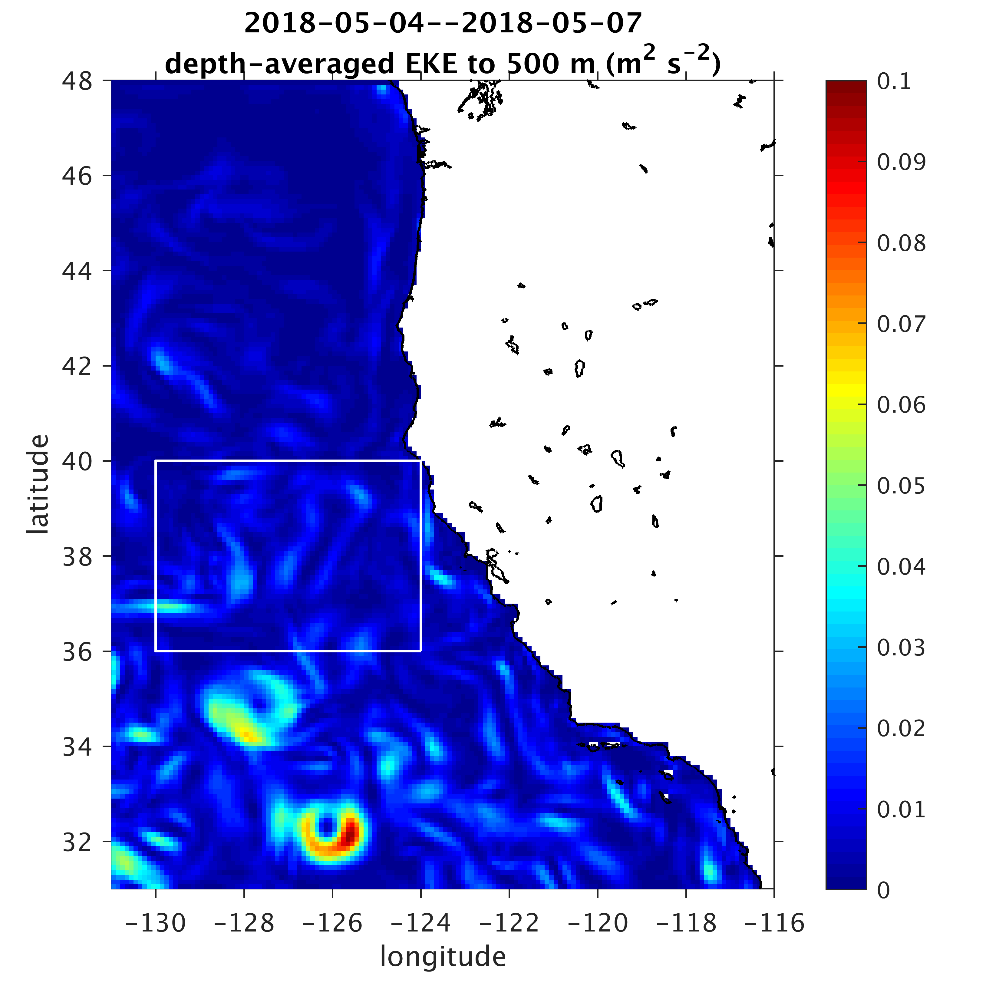
The Eddy Kinetic Energy (EKE) represents the energy in the difference between the horizontal ocean velocities and some mean background flow state, in this case a monthly climatology. This energy metric, 0.5(u′2 + v′2), is then averaged in time over each 4-day assimilation window and vertically from the surface to 500 m depth. An example for one cycle is shown below. Finally, the EKE is averaged horizontally within the white box below, an area of high eddy energy in the CCS during summer and fall.
The EKE evolves from cycle to cycle, as shown in the top panel below. The bottom panel reveals changes, or increments, in the metric due to the 4D-Var assimilation. Two estimates of the increments are given, one from a direct differencing of the prior and posterior model solutions (blue), and the other from the summation of all the individual observation impacts (red).

The impacts for different groupings of observation type are shown in the figure at the top of the page.
The Vertical Transport represents the net volume flux through an imaginary horizontal surface at 40 m depth. The metric is derived from the vertical velocity at 40 m. A time-average of the velocity for one 4-day cycle is shown below. The velocity at each ROMS grid cell is multiplied by the cell's area, and then the flux for all cells in the central California coastal region (within 50 km of shore, outlined in black) is summed to form a scalar metric.
The Vertical Transport evolves from cycle to cycle, as shown in the top panel below. The bottom panel reveals changes, or increments, in the metric due to the 4D-Var assimilation. Two estimates of the increments are given, one from a direct differencing of the prior and posterior model solutions (blue), and the other from the summation of all the individual observation impacts (red).
The impacts for different groupings of observation type are shown in the figure at the top of the page.
The Northward Transport represents the flux through an imaginary vertical surface extending along 37°N, from -127°E shoreward, and from the surface down to 500 m, or the bottom, whichever is encountered first. The metric is derived from the depth-averaged northward velocity at 37°N. A time-average of the velocity for one 4-day cycle is shown below. The northward velocity at each ROMS grid cell along 37°N is multiplied by the cell's width and thickness, and then the flux for all oceanic cells shoreward of -127°E is summed to form a scalar metric.
The Northward Transport evolves from cycle to cycle, as shown in the top panel below. The bottom panel reveals changes, or increments, in the metric due to the 4D-Var assimilation. Two estimates of the increments are given, one from a direct differencing of the prior and posterior model solutions (blue), and the other from the summation of all the individual observation impacts (red).
The impacts for different groupings of observation type are shown in the figure at the top of the page.

Density increases with depth in the ocean. The depth at which the density reaches a specific value can give insights into the ocean's circulation. The time average depth of the 1026 kg m-3 isopycnal for one 4-day cycle is shown below. This 2D map is averaged within the central California coastal region (within 50 km of shore, outlined in black) to form a scalar metric.

The Isopycnal Depth evolves from cycle to cycle, as shown in the top panel below. The bottom panel reveals changes, or increments, in the metric due to the 4D-Var assimilation. Two estimates of the increments are given, one from a direct differencing of the prior and posterior model solutions (blue), and the other from the summation of all the individual observation impacts (red).

The impacts for different groupings of observation type are shown in the figure at the top of the page.

The Energy Density represents the sum of the available gravitational potential and kinetic energy in the ocean. The metric is dominated by the available gravitational potential energy. This statistic gives the energy stored in the density structure of the ocean that could be converted into the kinetic energy of ocean currents. Near-surface values of the available potential energy for one 4-day cycle are shown below. The energy per unit volume is integrated over the entire model domain to give a scalar Energy Density metric.

The Energy Density evolves from cycle to cycle, as shown in the top panel below. The bottom panel reveals changes, or increments, in the metric due to the 4D-Var assimilation. Two estimates of the increments are given, one from a direct differencing of the prior and posterior model solutions (blue), and the other from the summation of all the individual observation impacts (red).

The impacts for different groupings of observation type are shown in the figure at the top of the page.
SST Mean Square Forecast Error
The accuracy of the forecast can be evaluated by specific metrics, such as the disagreement between the forecast and observed SST in the central California region, the black box in the figure below, which extends 200 km offshore. This error is shown for a particular 2-day forecast in September 2020 when the previous cycle is non-assimilative (prior case, top panel) and assimilative (posterior case, bottom panel).

The SST forecast mean square error evolves from cycle to cycle, and the effect of the assimilation on the error can be quantified by differencing the error of forecasts based on assimilative non-assimilative cycles. This difference is shown in the top panel below, where a negative value indicates the assimilation has improved the forecast (as in the figure above). Two estimates of the difference are given, one from a direct differencing of the prior and posterior model forecasts errors (blue), and the other from the summation of all the individual observation forecast impacts (red).
The forecast impacts for different groupings of observation type are shown in the bottom panel of the figure above.
SST Mean Square Forecast Error
The accuracy of the forecast can be evaluated by specific metrics, such as the disagreement between the forecast and observed SST in the central California region, the black box in the figure below, which extends 200 km offshore. This error is shown for a particular 2-day forecast in September 2020 when the previous cycle is non-assimilative (prior case, top panel) and assimilative (posterior case, bottom panel).
The SST forecast mean square error evolves from cycle to cycle, and the effect of the assimilation on the error can be quantified by differencing the error of forecasts based on assimilative non-assimilative cycles. This difference is shown in the top panel below, where a negative value indicates the assimilation has improved the forecast (as in the figure above). Two estimates of the difference are given, one from a direct differencing of the prior and posterior model forecasts errors (blue), and the other from the summation of all the individual observation forecast sensitivities (red).

The forecast sensitivity for different groupings of observation type are shown in the bottom panel of the figure above.
HF Radar Radials Mean Square Forecast Error
The accuracy of the forecast can be evaluated by specific metrics, such as the disagreement between the forecast and observed HF radar radial velocity in the central California region, the black box in the figure below, which extends 200 km offshore. This error is shown for a particular 2-day forecast in September 2020 when the previous cycle is non-assimilative (prior case, top panel) and assimilative (posterior case, bottom panel).

The HF radar radials forecast mean square error evolves from cycle to cycle, and the effect of the assimilation on the error can be quantified by differencing the error of forecasts based on assimilative non-assimilative cycles. This difference is shown in the top panel below, where a negative value indicates the assimilation has improved the forecast (as in the figure above). Two estimates of the difference are given, one from a direct differencing of the prior and posterior model forecasts errors (blue), and the other from the summation of all the individual observation forecast impacts (red).
The forecast impacts for different groupings of observation type are shown in the bottom panel of the figure above.
HF Radar Radials Mean Square Forecast Error
The accuracy of the forecast can be evaluated by specific metrics, such as the disagreement between the forecast and observed HF radar radial velocity in the central California region, the black box in the figure below, which extends 200 km offshore. This error is shown for a particular 2-day forecast in September 2020 when the previous cycle is non-assimilative (prior case, top panel) and assimilative (posterior case, bottom panel).
The HF radar radials forecast mean square error evolves from cycle to cycle, and the effect of the assimilation on the error can be quantified by differencing the error of forecasts based on assimilative non-assimilative cycles. This difference is shown in the top panel below, where a negative value indicates the assimilation has improved the forecast (as in the figure above). Two estimates of the difference are given, one from a direct differencing of the prior and posterior model forecasts errors (blue), and the other from the summation of all the individual observation forecast sensitivities (red).

The forecast sensitivity for different groupings of observation type are shown in the bottom panel of the figure above.
The Northward Transport represents the flux through an imaginary vertical surface extending along 37°N, from -127°E shoreward, and from the surface down to 500 m, or the bottom, whichever is encountered first. The metric is derived from the depth-averaged northward velocity at 37°N. A time-average of the velocity for one 4-day cycle is shown below. The northward velocity at each ROMS grid cell along 37°N is multiplied by the cell's width and thickness, and then the flux for all oceanic cells shoreward of -127°E is summed to form a scalar metric.
The Vertical Transport represents the net volume flux through an imaginary horizontal surface at 40 m depth. The metric is derived from the vertical velocity at 40 m. A time-average of the velocity for one 4-day cycle is shown below. The velocity at each ROMS grid cell is multiplied by the cell's area, and then the flux for all cells in the central California coastal region (within 50 km of shore, outlined in black) is summed to form a scalar metric.
Many people are responsible for various aspects of ROMS and the overall data assimilation code. Major contributors to UCSC data assimilation projects are listed below.
Andrew M. Moore
Hernan Arango
Hajoon Song
Milena Veneziani
Nicole Goebel
Christopher A. Edwards
Patrick Drake
Paul Mattern
Jerome Fiechter
Gregoire Broquet
James Doyle (NRL) has provided considerable assistance in our use of the COAMPS atmospheric fields.
We are also indebted to Brian Powell (UH) and John Wilkin (Rutgers) who have written and kindly shared outstanding scripts to carry out various ROMS-related operations.
- Veneziani, M., C. A. Edwards, J. D. Doyle, and D. Foley (2009), A central California coastal ocean modeling study: 1. Forward model and the influence of realistic versus climatological forcing, J. Geophys. Res., 114, C04015, doi:10.1029/2008JC004774.
- Veneziani ,M., C. A. Edwards and A. M. Moore (2009). A central California coastal ocean modeling study: 2. Adjoint sensitivities to local and remote forcing mechanisms. J Geophys Res, 114, doi:10.1029/2008JC004775.
- Broquet G., C. A. Edwards, A. M. Moore, B. S. Powell, M. Veneziani and J. D. Doyle, (2009), Application of 4D-Variational data assimilation to the California Current System, Dyn. Atmos. Oceans, doi:10.1016/j.dynatmoce.2009.03.001.
- Broquet G., A. M. Moore, H. G. Arango, C. A. Edwards, and B. S. Powell (2009), Ocean state and surface forcing correction using the ROMS-IS4DVAR data assimilation system, Mercator Ocean Quarterly Newsletter, Mercator Ocean Quarterly Newsletter, 34, pp. 5-13.
- Broquet, G., A. M. Moore, H. G. Arango, and C.A. Edwards (2010), Corrections to ocean surface forcing in the California Current System using 4D variational data assimilation, Ocean Mod. 36, doi:10.1016/j.ocemod.2010.10.005.
- Moore, A.M., Arango, H.G., Broquet, G., Powell, B.S., Zavala-Garay, J., Weaver, A.T., in press-a. The regional ocean modeling system (ROMS) 4-dimensional variational data assimilation systems. I: System overview and formulation. Prog. Oceanogr. doi:10.1016/j.pocean.2011.05.004.
- Moore, A.M., Arango, H.G., Broquet, G., Edwards, C.A., Veneziani, M., Powell, B.S., Foley, D., Doyle, J.D., Costa, D., Robinson, P., in press b. The regional ocean modeling system (ROMS) 4-dimensional variational data assimilation systems. II: Performance and application to the California current system. Prog. Oceanogr.doi:10.1016/j.pocean.2011.05.003.
- Moore, A.M., Arango, H.G., Broquet, G., Edwards, C.A., Veneziani, M., Powell, B.S., Foley, D., Doyle, J.D., Costa, D., Robinson, P., in press-b. The regional ocean modeling system (ROMS) 4-dimensional variational data assimilation systems: III Observation impact and observation sensitivity in the California Current system. Prog. Oceanogr. doi:10.1016/j.pocean.2011.05.005.
This web-page and the near-real-time ocean state estimation system is supported by the National Oceanographic and Atmospheric Administration (NOAA) through a grant from the Central and Northern California Ocean Observing System (CeNCOOS).We gratefully acknowledge financial support for various elements of this data assimilative system by the National Oceanographic Partnership Program (NOPP) , the Office of Naval Research (ONR), the National Oceanographic and Atmospheric Administration (NOAA) , the National Science Foundation (NSF), and the Gordon and Betty Moore Foundation .